The AVERAGE function in Excel calculates the average (arithmetic mean) of a group of numbers. The AVERAGE function ignores logical values, empty cells, and cells that contain text.

Average

Instead of the AVERAGE function, use the SUM and the COUNT function.

1. For example, the AVERAGE function below calculates the average of the numbers in cells A1 through A3.

2. The formula below produces the exact same result.

3. The following AVERAGE function calculates the average of the numbers in cells A1 through A3 and the number 8.

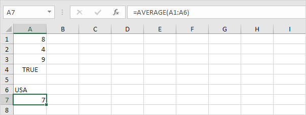
4. The AVERAGE function ignores logical values (TRUE or FALSE), empty cells and cells that contain text.

AverageA

The AVERAGEA function also returns the average (arithmetic mean) of a group of numbers. However, the logical value FALSE and cells that contain text evaluate to 0 and the logical value TRUE evaluates to 1. The AVERAGEA function also ignores empty cells.

1. For example, take a look at the AVERAGEA function below.

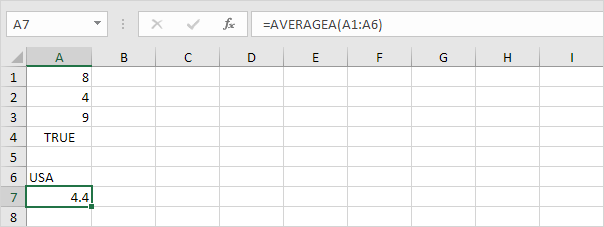
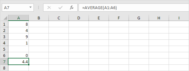
2. You can use the normal AVERAGE function to check this result.

Average Top 3

Use the AVERAGE and the LARGE function in Excel to calculate the average of the top 3 numbers in a data set.

1. First, the AVERAGE function below calculates the average of the numbers in cells A1 through A6.

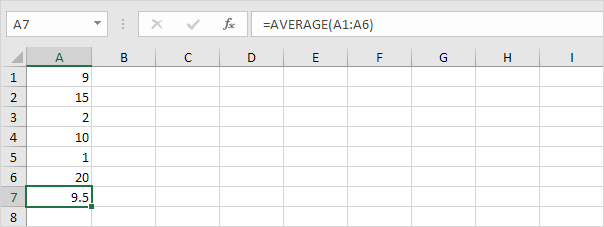
2. For example, to find the third largest number, use the following LARGE function.

3. The formula below calculates the average of the top 3 numbers.

Explanation: the LARGE function returns the array constant {20,15,10}. This array constant is used as an argument for the AVERAGE function, giving a result of 15.

AverageIf

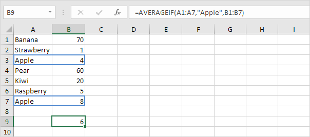
To calculate the average of cells that meet one criteria, use the AVERAGEIF function in Excel.

Weighted Average

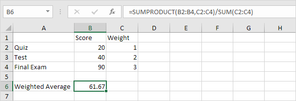
To calculate a weighted average in Excel, use the SUMPRODUCT and the SUM function.

Moving Average

Use the Analysis Toolpak to calculate the moving average of a time series in Excel.

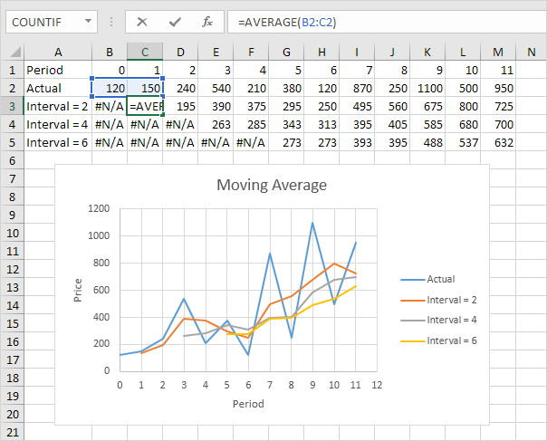
Note: a moving average is used to smooth out irregularities (peaks and valleys) to easily recognize trends.

How to Use Different Average Functions in Excel

In using Excel functions, you will certainly need to use the different average functions. In this article, we will explore the usages of all the average functions.

There are 4 variants of average functions: AVERAGE, AVERAGEA, AVERAGEIF and AVERAGEIFS. In the following part, we will talk about them in details.

1.    AVERAGE

AVERAGE function is used to calculate the average of a range. This function can also calculate the average of the arguments in formulas. Now we will use the example below to show the usage. In this image, you need to calculate the average of the sales volume.

1. Click a blank cell in the worksheet. Here we click the cell B14.
2. Now input the formula into the cell:

=AVERAGE(B2:B13)

The range in the formula contains the sales volume of the product “DataNumen Excel Repair”.

3. And then press the button “Enter” to move the cursor to other cell. And immediately you will get the result in the cell.

When it comes with multiple arguments in the formula, this function will calculate the average of all the arguments. Here it doesn’t mean that it will first calculate the average of every argument and then calculate the average of those average numbers. You can see the example below to see how it works.

1. Still we click the cell B14 in the range.
2. Now input this formula into the cell:

=AVERAGE(B2:B13,1)

3. And then you will get this result in the cell after you press the button “Enter”.

The result of the two arguments is “284.57”. It will not use the calculation formula “(308.2+1)/2” to calculate the average of those average numbers of arguments. Therefore, the next time if you use many arguments in this function, you need to be more careful about this key point.

2.    AVERAGEA

AVERAGEA can calculate the average of a range that contains logical values or text representations of numbers. And this is the difference between AVERAGEA and AVERAGE function. Here we will use a simple example to illustrate the usage. We will use the same worksheet that contains the sales volume.

In this image, there is a logical value “FALSE” in the cell B13. And we need to calculate the average of the range B2:B13.

1. Click a blank cell in the worksheet.
2. And then input the formula into the cell:

=AVERAGEA(B2:B13)

3. Next press the button “Enter” on the keyboard. Therefore, you will also get the result in the cell.

The formula in cell B14 is AVERAGE function. Thus, the results of the two functions are different. Because here the AVERAGEA will treat the “False” as 0, while the AVERAGE will not include the value in cell B13. Thus, when you need to calculate the average of a range with logical values or text representations of numbers, you need to use the AVERAGEA instead of AVERAGE function.

3.    AVERAGEIF

If you need to calculate the average of a range with certain criterion, you can use the AVERAGEIF function. Still we will use the worksheet that contains the sales volume. Suppose here we calculate the average of values and those values should be larger than 300.

1. Click a blank cell in the worksheet.
2. And then input this formula into the cell:

=AVERAGEIF(B2:B13,”>300″)

In this formula, the range and the average range is the same.

3. And then press the button “Enter” on the keyboard. Now you can check the result in the cell.

Besides, you can also use wildcard characters in the formula.

1. Click a blank cell in the worksheet.
2. Next input this formula into the cell.

=AVERAGEIF(A2:A13,”=J*”,B2:B13)

You want to calculate the average of months with the beginning “J”, thus you will use the character “*”. And the average range is B2:B13. Thus, you need to input it into the cell.

3. And then press the button “Enter” to move the cursor to other cell. Now you will also see the result in the worksheet.

4.    AVERAGEIFS

In AVERAGEIF function, you can only use single criterion. Sometimes you need to use multiple criteria to calculate the average of a range. Hence, you can use the AVERAGEIFS function. Now we will use this example to discuss about the usage.

1. Click a blank cell in the worksheet.
2. Next input this formula into the cell:

=AVERAGEIFS(D2:D13,B2:B13,”>300″,C2:C13,”>400″)

In this formula, there are two criteria. And the average column is the first argument in this formula. In your actual formula, each criteria range should have the same numbers of rows and columns. When all of the criteria are met, the cell will be calculated.

3. After that, press the button “Enter” again. Thus, you will get the result in the target cell.

In addition, you can also use wildcard characters in this function.

And for more practical application of the AVERAGEIF and AVERAGEIFS functions, you may also refer to our previous article How to Average Values Satisfying Specified Conditions with AVERAGEIF and AVERAGEIFS Functions.

The above are the details of all the average functions in Excel. When you need to calculate average, you can choose one of those functions according to your need.